Published in Fractals, Vol. 10, No. 3 (2002) 341-351

Some additions have been made to the paper published in the journal.

Yutaka Tachimori

Takashi Tahara　

Abstract

We examine the statistical properties of data concerning clinical diagnoses extracted from the medical database of our hospital. Specifically, we analyze all diagnoses given to all patients (inpatients and outpatients). The data consisted of both data input to computers as Japanese names, and the data input as ICD10* codes (International classification of Diseases 10^th Revision). We adapted the Zipf approach to analyzing the frequencies of clinical diagnoses for these two data groups. We found that both group types have the inverse-power relationship between the rank order of diagnoses and the frequency of the appearance of these diagnoses (This relationship is called Zipf’s law, which is observed in natural language). Though the reason why these sets follow Zipf ’s law is unknown, we speculate that the complex interaction between doctor and patient is the cause for adherence to Zipf ’s law.

* : The International Classification of Diseases is a system of categories for classifying various forms of morbidity. The ICD is designed to facilitate the statistical study of disease phenomena.

1. Introduction

  In medical treatment, clinical diagnosis can be viewed as the most basic piece of information. When a doctor examines a patient, the first task is to determine the clinical diagnosis. Then, the doctor can proceed with medical treatment based on that diagnosis. For hospital management, coded diagnoses are very important. Changes in the frequencies of diagnoses are important from the perspective of medical policy and budget making. However, it has been difficult to find investigations regarding the frequency distribution of diagnostic data. In this study, we found that the frequencies of clinical diagnoses have certain statistical features in common with natural languages.    As for natural languages, it is known that the frequencies of words follow what is called Zipf ’s law [1-3].  To apply this law, one calculates the frequencies of words within a given text. If all the words in the text are arranged in rank order, from most frequent to least frequent, an inverse power-law relation holds between the frequencies and the rank of the frequencies. The frequency of the word F_n, which has the rank n, is expressed by the following equation,  

where A is constant. In this equation z is referred to as Zipf exponent, and in natural languages the exponent z was found to be close to one. In other words, log-log plots of the frequency versus rank show a linear relationship between these two variables. This relation is called Zipf ’s law. This law holds not only for languages, but also formany situations (e.g., the population of cities and their rankings)⁴.  In particular, it was recently discovered that DNA sequences have the same linguistic features [5-12]. 

  Our objectives were to determine whether the frequencies of clinical diagnoses follow Zip’s law and to investigate the influence of coding diagnoses on the distribution of frequencies.

2. Methods

  We analyzed data regarding the diagnoses stored within the database of Toyonaka Municipal hospital. We analyzed two data sets separately; one is the set of diagnoses written on charts before October 1997, and the other is the set of diagnoses input into a computer after November 1997. The diagnoses before October 1997 were input on the computer by clerks, using the Japanese names on the charts of patients who had received medical advice even once within the one year period before October 1997. These data were input as Japanese text without code. Therefore, several names that indicate the same disease may be entered as different names due to differences in writing. Moreover, there is a likelihood of an error upon input or miswriting on a chart, and in these cases, we input this erroneous name as a new different name. We think that the probability of making the same error twice is low, and in this case, the frequency of that diagnosis only amounts to one. A considerable number of the diagnoses showing a frequency of one is thought to be obtained by such errors and so we excluded all diagnoses showing a frequency of one from our analysis. The diagnoses were written on charts between July 1953 and October 1997. The total number of patients was 39,212 and the total number of diagnoses was 101,760, so the average was 2.6 diagnostic names per patient. Henceforth, we call this group the “freely written group”.

   The second group of data was collected between November 1997 and October 1998, and these data were directly input by doctors during this period. These data were basically input in the form of name codes that are registered as master data in the computer. Doctors input the Japanese name itself only when they did not find a corresponding name code. Entered name codes consist of six characters and the first four characters are the ICD10 codes (International classification of Diseases 10^th Revision). The last two characters are Toyonaka’s own additional coding characters. With this additional coding, we can provide a more detailed categorization than ICD10 code alone. A correspondence map between this code and the Japanese disease name is registered as master data in the computer. By choosing a Japanese name on the computer, a doctor can input data with its code. Both code and the Japanese name are entered in the database file as the clinical diagnosis. In the present study, we used only the name codes for analysis. Some data did not have codes, and we have not used such data here. The total number of patients was 47,964 and the total number of diagnoses was 137,933, so the average was 2.9 diagnoses per patient. Data that had no diagnosis codes comprised 3.3 % of all data, and were excluded from further analysis. Henceforth, we call these data the “coded group”.

  We analyzed all data from all patients (inpatients and outpatients). With regard to a particular patient (and their initial diagnosis), the diagnosis (i.e., the name of the disease) may change after the first medical examination based on more detailed medical tests. However, we counted all diagnoses as distinct data.

  We evaluated the frequencies of clinical diagnoses for each group and the rank of each diagnosis (the most frequent diagnosis has the rank of one; the second most frequent diagnosis has the rank of two, and so on.). Moreover, we plotted a logarithm of the frequency versus a logarithm of the rank (Zipf plot [7]⁷). In the freely written group, we defined two names (Japanese names) as the same if and only if all characters contained in each diagnosis were completely identical (e.g., “Gastric Cancer” and “Cancer of Stomach” are regarded as different diagnosis). Therefore, we sometimes counted two diagnoses indicating the same disease as different ones only due to differences in the description.

In order to investigate the details of the distribution, we classified each data set into subgroups according to departments from which patients received medical advice and attention. Furthermore, with respect to the coded group, we also classified these data into subgroups according to doctors. These subgroups were also analyzed using a Zipf plot.

3. Result

3.1 Freely written group

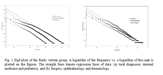
  Figure 1 shows the result of the Zipf plot in the freely written group. In this figure (and these plots, in general), the X-axis denotes the logarithm of the rank of frequencies, and the Y-axis denotes the logarithm of frequencies. Moreover, regression lines for each data set are also expressed in the figures. For all departments, the data are fitted well by regression lines. These results mean that for all departments, the data follow Zipf’s law.  However, at high frequencies (from rank 1 to 10, i.e. from 0 to 1 in X-axis) the data deviate less from the regression lines. These deviations are large in the “total diagnoses” group and in the internal medicine group. Causes of these deviations, especially among the total diagnoses and the internal medicine groups, will be discussed in the next section. Table 1 shows slopes of the regression lines for some departments and for the total set. In the freely written group these slopes are close to one.

3.2 Coded group

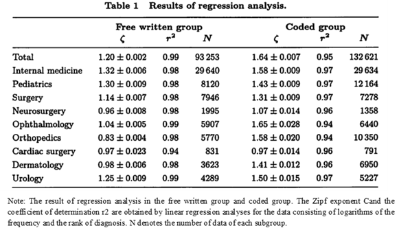
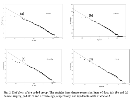
For all groups except the total diagnoses and the internal medicine groups, data are fitted well by Zipf ’s law, especially at the low frequency regions (Fig. 2a-c). As shown in the fig. 2d, subgroups corresponding to doctors are also fitted well by Zipf’s law. However, for internal medicine and total diagnoses, data points deviate considerably from the predicted straight lines (Fig. 3). The deviations from straight lines at high frequencies are larger than those in the freely written group. These phenomena will be described in detail later.

4. Discussion

4.1 The Union of Zipf sets causes the deviation

We indicate that in almost all groups, the distribution of clinical diagnoses is fitted well by Zipf ’s law. However, in analyzing thedetails of the results, we can recognize the deviation from Zipf’s law at high frequencies.

We begin by considering the result obtained from the present study. A diagnostic set of a certain department(e.g., surgery, pediatrics, etc.) is the union of diagnostic sets of all doctors who belong to this department. From the present results, the sets of doctors are Zipf sets (Zipf set indicates a set that follows Zipf’s law), and the union of these sets (i.e., the set of the department) is also Zipf set. This fact suggests that the union of several Zipf sets is also a Zipf set. Similarly, the total set of the hospital is the union of sets of all departments and the total set is also Zipf set. Moreover, the deviation at high frequencies of the total set is great compared to those of the sets of individualdepartments.  This observation suggests that the union of Zipf sets has the great deviation at high frequencies compared to the original Zipf sets.

  We next consider a simple mathematical example.

Example: Suppose two sets of equal size, which have no common diagnosis, and follow Zipf’s law with a Zipf exponent of 1. For instance, data sets from ophthalmology and urology satisfy this condition. We suppose the numbers of diagnoses are both N. Combining the two sets, the number of diagnoses amounts to 2N. If two sets have the same distribution and do not have any common diagnosis, the diagnosis with rank n in the source sets will have the rank 2n(=K) or the rank 2n-1 in the unified set. This frequency is A/n (A is constant). Thus, the frequency Y_K for the diagnosis with rank K in the new set is expressed in terms of the following equation: Y_K =Y_2n =A/n=2A/2n=2A/K=Y_2n-1=Y_K-1. Therefore, for a large n, Y_K asymptotically approaches Zipf’s law, and has the same Zipf exponent as the source sets. However, at high frequencies (in other words, where K is small), it deviates from Zipf’s law.  Figure 4 shows the Zipf plot of the union of five sets with no common diagnoses. At low frequencies, we can see that the data are well fitted by a straight line. However, at high frequencies, data deviate from the expected line with the data points falling below the line.

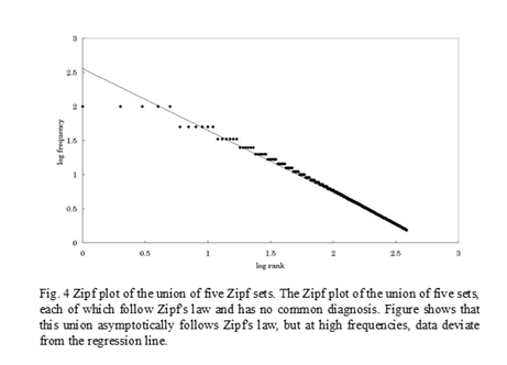
This simple example indicates that the union of several sets, which follow Zipf ’s law and have no common diagnosis, is asymptotically fitted by Zipf ’s law. However, at high frequencies, such sets will deviate from Zipf ’s law. 

This theoretical consideration, as well as the results obtained from the present data, indicates that the union of several Zipf sets is one of causes of the deviation from Zipf’s law at high frequencies. Moreover, this suggests that the sets of diagnoses for this analysis (total set of diagnoses, sets of each department, and sets of each doctor) consist of the union of some smaller subgroups, each of which follows Zipf ’s law.

In the analysis of the coded group, the deviations from straight lines at high frequencies are larger than those in the freely written group, especially in internal medicine and the total set of diagnoses. This suggests some other cause in addition to the union of Zipf sets.A possible cause is the saturation of diagnoses, which indicates the situation that the number of unused diagnoses decreases due to having used many names. In the coded group, the number of usable diagnoses is limited to the number of codes that are registered. The number of master data being used at this time is about 12,000. If the number of names used for patients increases to approaching the upper limit in the master data, it is possible that the saturation of diagnoses causes a deviation from Zipf ’s law. In case of the total set of diagnoses, the number of diagnoses used is over 3,200, so it is possible that the influence of the saturation of diagnoses is shown.

4.2. The set of clinical diagnoses consists of “element sets” (Additional text in this paper)

The second feature of the data is that the Zipf exponents of the coded group are larger than that of the free written group. Now we consider whether coding causes this fact. Compared to names expressed in terms of code, in the free written group, fluctuation of writing gives rise to many different diagnoses that indicate the same disease. So, this group contains more diagnoses than the coded group. Namely, coding means combining several names of one disease under one code. Conversely, each coded name of a disease can be broken up into several names. We considered how the distribution of the diagnoses sets would change when each name in it was divided into several new names. At first we assume that one coded name is broken up into a fixed number of names and the frequencies of new names are the same. In these cases, the new diagnoses set follows Zipf ’s law but the Zipf exponent does not change. This is indicated the same way as proving that combining two Zipf sets without common data yields a new Zipf set with the same Zipf exponent. Secondly, we assume that a set, which is constructed by dividing one name into several names, also follows Zipf ’s law. We are not sure why a word’s distribution in writing follows Zipf ’s law, but it is possible that this distribution is produced by the free choice of one word from many words with the same meaning. Therefore, in the case of the free written diagnoses, the same principle appears to cause Zipf ’s law.

   We considered a set of coded names. We assume that frequency F_x is expressed as follows:

where A is constant, x denotes the rank of a diagnosis and [ ] denotes “rounding off fractions”.    We also assume that a set produced by dividing one name into several names follows Zipf ’s law with Zipf exponent=1. The sum of the frequencies of elements of this set equal F_x, which results in the following equation:

where B is constant and n denotes the number of new diagnoses. We try to calculate B and n as follows. Because the lowest frequency of a diagnosis is one, B and n satisfy the equation:

Substituting B = n into Eq. (1), we can obtain

so, we determine n to satisfy following condition.

Then, we can find s satisfying the following formula.

In the right side of this formula, factor 1 is added so that we can always determine s. In the absence of factor 1, there are cases where the right side does not reach the left side. In this way, we divide the set of diagnoses of rank x into s subgroups. And we obtain a new set of diagnoses by dividing all the diagnoses in the same way. What is the distribution of this new set?   We show the change in distribution by simulating the above procedure. In that simulation, we use data satisfying the condition F₁ = A =10000 in Eq. (1). This original data has Zipf exponent z= 0.97. The new set obtained by dividing each diagnosis into several new diagnoses has 19,685 names and follows Zipf’s law with Zipf exponent z=0.67 (Fig. 5).

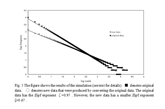
This simulation shows that the division of a set of diagnoses into subgroups, each of which follows Zipf’s law, yields a new set which follows Zipf’s law with a smaller Zipf exponent. Inversely, coding is thought to be the process in which we regard a group of diagnoses following Zipf’s law as one diagnosis. If this is true, the Zipf exponent is expected to increase by coding. We checked this hypothesis using actual data. In the present study, we use codes of diagnoses consisting of six characters: four ICD10 codes and two additional codes. So, we checked the distribution of the new diagnosis set obtained by distinguishing only four ICD10 codes (e.g., two codes “A12345” and “A12378” are regarded as the same). As a result, we found that this conversion of diagnoses gives rise to a new Zipf set which has a larger Zipf exponent, confirming our hypothesis.

In the analysis of the coded group, the set of diagnoses of internal medicine and the total set of diagnoses show a large deviation from Zipf ’s law, especially at high frequencies. We consider why this has occurred. At first, internal medicine contained the most varied diagnoses compared to those of other department. This suggests that the diagnosis set of internal medicine is composed of the union of many sets compared to other department. As described above, the union of several Zipf sets without common diagnoses yields a new set which asymptotically follows Zipf ’s law, but the Zipf plot deviates from a straight line at high frequencies. In internal medicine, it is possible that because of the union of so many sets, the diagnosis set deviates considerably from Zipf ’s law at high frequencies. The same situation is thought to be responsible for the total set of diagnoses. Another possible cause is the saturation of diagnoses, which indicates the situation that the number of unused diagnoses decreases due to having used many names to express the same disease. In the coded group, the number of usable diagnoses is limited to the number of codes that are registered. The number of master data being used at this time is about 12,000. If the number of names used for patients increases to approaching the upper limit in the master data, it is possible that the saturation of diagnoses causes a deviation from Zipf’s law. In case of the total set of diagnoses, the number of diagnoses used is over 3,200, so it is possible that the influence of the saturation of diagnoses is shown.

 In the present study, we obtain several sets of clinical diagnoses by categorizing diagnoses according to many standards (e.g., department, doctor, and ICD10 code), and all the sets followed Zipf’s law. Considering the fact that many sorts of categorization yielded Zipf set and the union of Zipf sets asymptotically follows Zipf’s law again, it is possible that Zipf’s law holds at the level of smaller sets than that used in the present study. If so, we can say that all the sets for the present analysis are obtained by the union of small Zipf sets (we call them “element sets”) and, of course, follow Zipf’s law again. To prove the existence of such element sets, it is necessary to make a model using a constructive approach to showing how a set of clinical diagnoses is produced and to analyze that [4][17].

4.3 Giving a clinical diagnosis depends on context

    The clinical diagnoses are not all independent of each other. Some diagnoses are strongly dependent on another, while other diagnoses are independent. For example, suppose there is a patient who shows symptoms of a common cold. It is possible that a doctor diagnoses his illness as one of following diseases: common cold, upper respiratory infection, acute rhinitis, acute pharyngitis or acute bronchitis. These names are easy to shift (or to diagnose in error) from one to another. In this sense, it is thought that these are closely related to each other, in other words, the distance between them is short. However, we do not think femoral fracture and upper respiratory infection can be confused, so we think that these two diagnoses are not related and the distance between them is great. Of course, the distance between two diagnoses depends on the measures with which a doctor examines a patient. There are many measures that affect diagnosis: e.g., measures based on cause, on symptoms, on the degree of seriousness, and on the social influence. When a doctor examines a patient, he uses different measures depending on the situation (initial examination, a special test, patient’s social standing, midway through treatment, etc.). However, we think that whenever a doctor examines a patient, he certainly uses some kind of measure. At this time, his diagnosis name may shift to another close name depending on the measure. We speculate that the set of diagnoses, which is obtained by collecting these closely related names, follows Zipf ’s law.

  For instance, we consider a situation that all of several close diagnoses fit the symptoms of a patient, but there is no absolute standard for selecting one of these due to the vagueness that the each diagnosis has. In such cases, the selection of the diagnosis depends on the doctor’s free choice. This situation is similar to a situation in which we select one from many possible words when we write a composition. So, we think that a set of closely related diagnoses follows Zipf ’s law and it may be a candidate of the “element set”.

  A doctor examines a patient, and as a result he determines the diagnosis. On this occasion, this determination is influenced by the expertise of the doctor, the instrument used for tests, the state of the patient and so on. This fact suggests that the diagnosis is the result of an interaction between the doctor and patient rather than objective existence. So it is possible that with the changing status of the doctor, the resultant diagnosis even for the same patient may change. This suggests that the distribution of diagnoses also varies by changing the status of the doctor (in other word, changing the method of observation). These diagnoses are generated by various observations. We can consider two extremely different types of observations. One is an ordinary medical examination, in which a doctor chooses one diagnosis from a nearly infinite list of possibilities based on the complaints and the state of the patient. The other is the observation such as that during an examination for cancer. In this case, a doctor chooses one diagnosis from a few diagnoses fixed beforehand or the diagnosis “no disorder”. If we perform these two observations for a group of the same patients, frequencies of diagnoses may be much different.

In a set that follows Zipf ’s law, the frequency of a certain element depends on the size of the set. And the average and dispersion of frequencies over the total set also depend on the size. The dispersion of frequencies diverges to infinity with the size of the set, when the Zipf exponent is small than 2. This situation is not ordinarily accepted. However, in the present study, we indicate that frequency may change with changes in the method of observation. This may show that the measure of “the frequency of a diagnosis” obtained by extension of the frequency of a sample does not originally exist. This is similar to the situation in which the idea “a curve without length or a plane without area” arises from the discovery of “Fractal” [16].

4.4 Many medical indices also follow Zipf’s law

   Though we do not present the data at this time, in addition to the clinical diagnoses, medical indices such as average length of hospital stay, frequencies of medical treatments expressed in terms of ICD9-CM (International Classification of Disease 9^th Revision, Clinical Modification), and medical fees, also follow Zipf’s law. These facts suggest that not only the clinical diagnoses but also the medical structure itself is based on complex interactions between patients and a medical system that includes a medical team, medical facilities, and medical equipment, and all of these interactions yield Zipf ’s law. A more detailed study of the health care delivery structure on the basis of the theory of complex systems is required.

5. Conclusion

It was proven that the diagnostic sets based on the doctor’s diagnoses followed Zipf’s law. This indicates thatthe diagnostic set is a set interactively created by the doctor, patient, and hospital, and it follows a certain order called Zipf’s law. This fact indicates that the medical system, consisting of doctor-patient interaction, is a so-called complex system. Furthermore, the indication that diagnostic sets observe Zipf’s law may possibly have major effects on changing the conventional concept of diagnostic frequency rate.

Acknowledgement

  The authors would like to thank Professor I. Tsuda (Hokkaido University), H. Takayasu (Sony Computer Science Laboratories, Inc.), and Y. Hirota for their useful discussion.

Reference

[1]       J.L. Casti, “Bell curves and monkey languages,” Complexity 1(1), 12-15 (1995).

[2]       G.K. Zipf, “Human Behavior and the Principle of Least Effort,” (Cambridge Mass, Addison-Wiesley, 1949).

[3]       D.R. Ridley and E.A. Gonzales, “Zipf’s law extended to small samples of adult speech,” Percept. Mot. Skills. 79, 153-154 (1994).

[4] A.S. Iberall, H. Soodak and F. Hasslerm, “A field and circuit thermodynamics for integrative physiology. II. Power and communicational spectroscopy in biology,” Am. J. Physiol. 234, R3-19 (1978).

[5]       R.F. Voss, “Evolution of long-range fractal correlations and 1/f noise in DNA base sequences,” Phys. Rev. Lett. 68, 3805-3803 (1992).

[6]       R.N. Mantegna and S.V. Buldyrev, A.L. Goldberger and et al. “Linguistic features of noncoding DNA sequences,” Phys. Rev. Lett. 73, 3169-3172 (1994).

[7]       R.N. Mantegna, S.V. Buldyrev, A.L. Goldberger and el al. “Systematic analysis of coding and noncoding DNA sequences using methods of statistical linguistics,” Phys. Rev. E. 52, 2939-2950 (1995).

[8] J.D. Burgos and P. Moreno-Tovar, “Zipf-scaling behavior in the immune system,” Biosystems. 39, 227-232 (1996).

[9] B.J. Strait and T.G. Dewey, “The Shannon information entropy of protein sequences,” Biophys. J. 71, 148-155 (1996).

[10] J.D. Burgos, “Fractal representation of the immune B cell repertoire,” Biosystems. 39, 19-24 (1996).

[11] C.A. Chatzidimitriou-Dreismann, R.M. Streffer, D. Larhammar and et al. “Lack of biological significance in the ‘linguistic features’ of noncoding DNA－a quantitative analysis,” Nucleic. Acids. Res. 24 (9), 1676-1681 (1996).

[12] A.A. Tsonis, J.B. Elsner and P.A. Tsonis. “Is DNA a language?” J. Theor. Biol. 184 (1), 25-29 (1997).

[13] J.S. Nicolis and I. Tsuda, “On the Parallel between Zipf’s Law and 1/f Processes in Chaotic Systems Possessing Coexisting Attractors,” Prog. Theor. Phys. 82(2), 254-273 (1989).

[14] L.A. Lipsitz and A.L. Goldberger. “Loss of ‘Complexity’ and Aging Potential Applications of Fractals and Chaos Theory to Senescence,” JAMA. 267, 1806-1808 (1992).

[15] P. Bak, C. Tang and K. Wisenfeld, “Self-organized criticality,” Phys. Rev. A. 38, 364-374 (1988).

[16] B.B. Mandelbrot, “The stable Paretian income distribution when the apparent exponent is near zero,” Int. Econ. Rev. 4, 111-115 (1963).

[17] B.B. Mandelbrot, “The variation of certain speculative stock prices,” J. Bus. 36, 394-419 (1963).

[18] B.B. Mandelbrot, “New methods in statistical economics,” J. Polit. Econ. 71, 421-440 (1963).

[19] B.B. Mandelbrot, “The Fractal Geometry of Nature,” (New York, Freeman, 1983).