Chaotic pulsation in human capillary vessels and its dependence on the mental g physical conditions

Ichiro Tsuda, Takashi Tahara*, Hiroaki Iwanaga⁺
International Journal of Bifurcation and Chaos, Vol. 2, No. 2 (1992) 313-324

Department of Artificial Intelligence, Faculty of Computer Sciences, Kyushu Institute of Technology, Iizuka 820, Japan,
* Hizen National Mental Hospital, Kanzaki, Saga, 842-01, Japan,
+ Section of Research and Development, Computer Convenience Inc., Hakata 3-6-1, Fukuoka 812, Japan

Abstract
We found a chaotic pulsation in a finger’s capillary vessels in both normal subjects and psychiatric patients, as well as a cardiac chaos. A proof of chaos was made by the reconstruction of dynamics in phase space and the calculation of the Lyapunov exponents. From the aspect of chaotic information processing we give a measure of the information storage capacity of observed chaos. We also found a difference in the topology of capillary and cardiac chaos, and a difference in their dependence on the subject’s conditions.

1. Introduction

The recent development of dynamical systems’ theory enables us to interpret systematically complex behaviors in physical and even in biological systems. In particular, the technique of embedding [Packard et al., 1980;Takens, 1981] of observed data into finite or infinite dynamical systems may force a change in the analysis of random motions. Namely, before the development of such a technique, one tried to calculate average, standard deviation and, if necessary, higher moments of an observed random variable as well as a probability distribution function. Whereas, in the present, one may try to analyze random motions as an entity, not as a decomposed one as above, by extracting an implicated order in the form of nonlinear smooth manifold, i.e., geometry [Campbell et al.,1987].

By the embedding technique, the presence of deterministic chaos has been clarified in many complex systems. In particular, evidence of deterministic chaos in human brain and heart has been obtained in several experiments by adopting this technique to the data of electro-encephalogram (E.E.G.) [Babloyantz, 1986; Layne et al., 1986 ; Rapp et al., 1989] and electro-cardiogram (E.C.G.) [Babloyantz, & Destexhe, 1988; Goldberger et al.,1988].

In this paper, we present another human chaos: the capillary chaos. Furthermore, recent studies on applications of dynamical systems’ theory to biological systems raise expectations of the discovery of novel indications for the process of recovery of health. Such appropriate indications could be utilized in care and cure [Rapp,1986]. It is worth studying correlation of the peripheral data with controlled conditions by reconstructing the dynamics of the peripheral, since the peripheral activities vary easily for a change of mental or physical conditions.

One of the crucial problems for human brain is how to get an indication for recovery of mental health, i.e.,care and rehabilitation problem. The present study is motivated to find a good indication for rehabilitation of a psychiatric patient This also leads to a study of the peripheral. If the patient could be aware of his current condition by means of an appropriate indication that should be simple and in particular, appearing as a visual image, such an indication would be available for the process of healing and rehabilitation. This notion could be generally applied to daily health-care.

Motivated by this fundamental notion of self-care, we recorded time series of pulsation of the capillary vessels, and we found chaotic pulsation in a finger’s capillary vessels in both normal subjects and psychiatric patients. We observed the geometry of an attractor constructed from time series of a single variable, i.e., the peripheral blood pressure, and we also calculated the Lyapunov exponents from the experimental data, which can express the degree of orbital instability. The results proved deterministic chaos. Forms of the chaos depended on the mental or physical conditions of the subjects.
We also studied the ability of observed chaos of detecting information fed from outside. This ability was measured by mutual information.

Furthermore, cardiac activities, i.e,, beating of the heart simultaneously measured by electro-cardiograph with a pulsation of the capillary vessels also exhibited deterministic chaos, whose forms were, on the contrary, almost independent of the subjects condition. This leads us to propose a hypothesis on the autonomic nerve innervation.

In Sec. 2 and Sec. 3, we explain the experimental system and the reconstruction technique, respectively. In Sec. 4, we give the computation results of the Lyapunov exponents, adopting the Wolf method[Wolf et al., 1985]. The condition dependence of the capillary and the cardiac chaos is given in Sec. 5. A measure for information processing of observed chaos is given in Sec. 6. Section 7 is devoted to discussions and outlook, with some hypotheses.

2. Experimental system

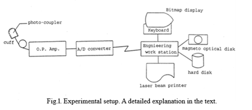
The data were recorded from the surface of the bulb of the left forefinger by detecting light reflected by the vascular tissues of the infrared ray emitted from the Light Emitting Diode(LED). The setup of the experiment is drawn in Fig. l. The peripheral blood pressure was measured by the photo-coupler attached to the inner surface of the cuff which fixed the measurement place. The light with wavelength 940 nm emitted from the infrared LED was reflected from the vascular tissues and detected by the photo-transistor. Detected light intensity which was transformed to electric signal by the photo-transistor was stored in an engineering work station through the A/D converter (after being amplified by 10,000 times) where we measured the data with a sampling frequency of 200 Hz with 12 bit resolution.

A forefinger of the left hand was consistently chosen for all subjects. In the present experimental system, one can detect almost the same output for other seven fingers, but the thumbs exhibit a slightly different data set.

If the finger cannot move, a variable part in the data is reasonably derived from the motion of the blood flow. It is, however, questionable if we could remove the effect of the motion of the bulb. To check this, another measurement was made, where the data were taken on the surface of the nail. The result was the same, except for a slight decrease of the output intensity. Though we cannot determine the precise spatial extension of the measurement place, it will be a plausible estimation that it is within a few millimeter square. Thus, the apparatus can measure the time series of the collective pulsation of the capillary vessels, namely, the peripheral blood pressure. The data were taken from 20 normal subjects and 15 psychiatric patients.

3. Reconstructing dynamics

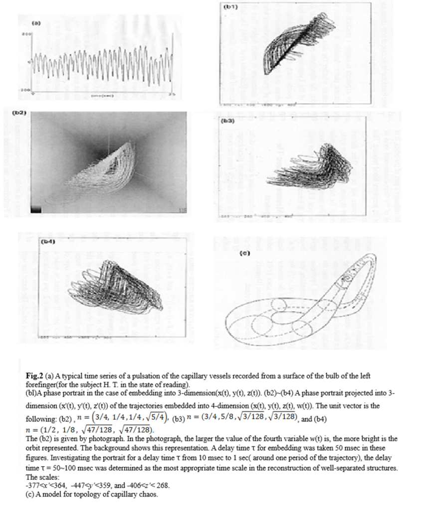
A typical time series is shown in Fig. 2(a). An oscillation with a period about 1 second is dominant, whose period is a reflection of the cardiac activities. In a long time observation (about 100sec. in the present case), however, both amplitude and period fluctuate over rather wide range. We reconstructed the attractor from these experimental data, by adopting the method of embedding.

For a variable \(x(t)\) denoting a time series of the peripheral blood pressure, we take new variables \(y(t)=x(t+\tau), z(t)=x(t+2\tau), w(t)=x(t+3\tau), \cdots,\) where \(\tau\) is the order of correlation time. In the embedding into three-dimensional phase space(Fig.2(bl)), we observed some complicated structure of the reconstructed attractor, but we could not obtain a consistent topology with possible vector fields of three-dimensional dissipative dynamical systems. This indicates that at least the fourth dimension is needed to satisfy the topological consistency, so we tried to make the embedding into four-dimensional phase space \([x(t), y(t), z(t), w(t)]\). We analyzed qualitatively the geometry of the attractor projected into three-dimensional phase space \([x'(t), y’(t), z’(t)]\), by taking the parallel projection[Miyazaki, 1989 ] of a supposed four-dimensional object.
The prqjection is given by Eq. (1),

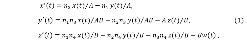
where \(A=(n_1^2+n_2^2)^\frac{1}{2},\ B=(1-n_4^2)^\frac{1}{2}, \ and\ \boldsymbol{n}=(n_1,\ n_2,\ n_3,\ n_4)\) is a unit vector representing the direction of sight. The fourth axis \(w\) was rotated to coincide with the direction of that unit vector. A typical phase portrait is shown in Fig.2(b2)~(b4).

Fig,2(c) shows a possible model for the geometry of the attractor. This is inferred by varying the direction of sight \(\boldsymbol{n}\) and observing the shape of the attractor on the three-dimensional Poincare maps: three-dimensional solid torus with a screw type of structure of torus as a part. If one tries to make a model with topological dimension 2, two singularities appear. To remove singularities, at least one more topological dimension is needed. A dotted line with arrows in the model indicates a part of orbits. A similar model in the four-dimensional embedding has been also proposed in the local E.E.G. of mammalian brain [Freeman 1989; Yao&Freeman 1990].

4. A pragmatic measure of chaos: the Lyapunov exponent

We did not succeed in determining a dimension of the attractor(eg. the correlation dimension[Grassberger & Procaccia, 1983(a)&(b)] ) directly from the experimental data. Since the observed attractors are very much nonunifbrm, conventional methods for the measurement of attractor*$ dimension such as the Grassberger-Proccacia method are inappropriate for our attractors. In general, even when the overall attractor is nonuniform, the Grassberger-Proccacia method is applicable to the Poincare sections if uniformity of invariant density on the sections is presumed[Schaffer et al. 1988].In the present case, however, it was practically impossible, because of the difficulty to record indefinitely many data of the peripheral blood pressure, assuring its stationarity. The maximum number of data we could record was about 20,000 sampling points by the measurement with 5msec sampling time. This number is too small to assure the invariance of the probability density of orbits on 3-dimensional Poincare sections. Furthermore, the correlation dimension may become fractional also in the case of non-chaos, for instance, colored noise, stochastic process like Levy flight, etc.

The Lyapunov exponent is simply a practical measure of deterministic chaos* Actually, it is undecidable to determine whether the data are chaotic or not. Furthermore, the algorithms proposed so far for the estimation of the Lyapunov exponents also have decisive weak points such as impossibility of discrimination of chaos and noise, and possibility of the appearance of spurious positive exponents when the embedding dimension is much higher than the system’s dimension[Eckmann et al.,1986]. The latter becomes destructive if the system’s dimension is not known in advance. Actually, this is decisive in the case of highly nonuniform attractors, in which the precise estimation of correlation dimension is hopeless such as in the present case.

These difficulties appear, particularly, in the estimation of exponents other than the largest one. The estimation of the largest exponent is relatively reliable, since the arbitrarily chosen vector quickly tends to the direction of the unstable manifold. This is a reason why we took here the Lyapunov exponent as a practical measure of deterministic chaos.

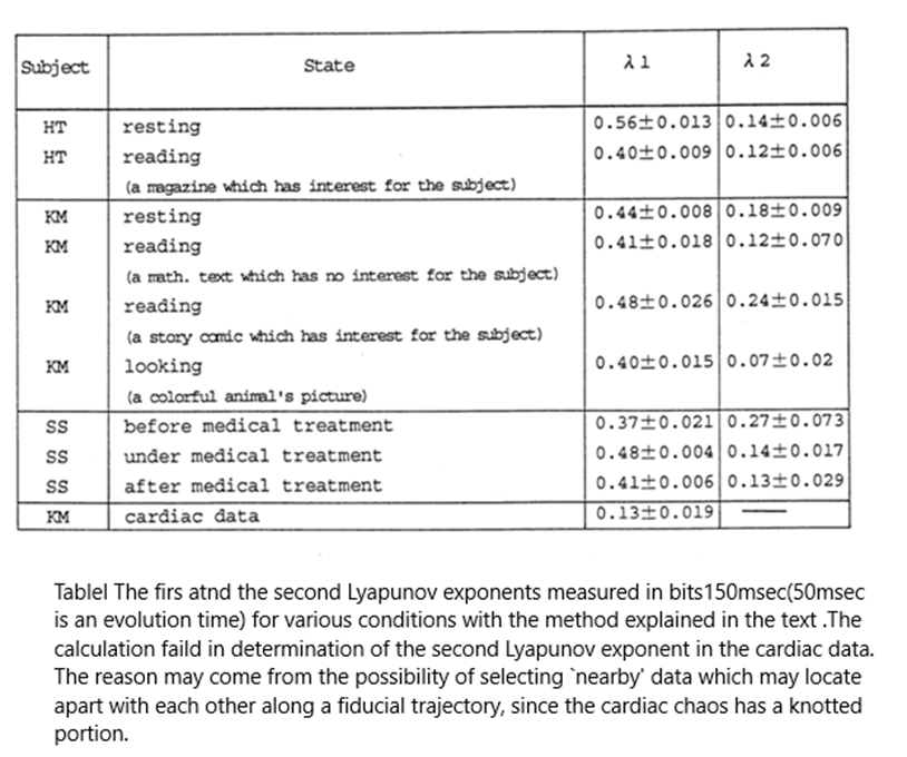
The calculation of the Lyapunov exponents from the experimental data showed the presence of a positive exponent The results are summarized in Table 1. We calculated the Lyapunov exponents with the Wolf method (Fig.3). The number of the present data is greater than, but close to the theoretical lower bound of the number of the data needed to estimate a correct value of the Lyapunov exponent in the case of four-dimensional embedding.

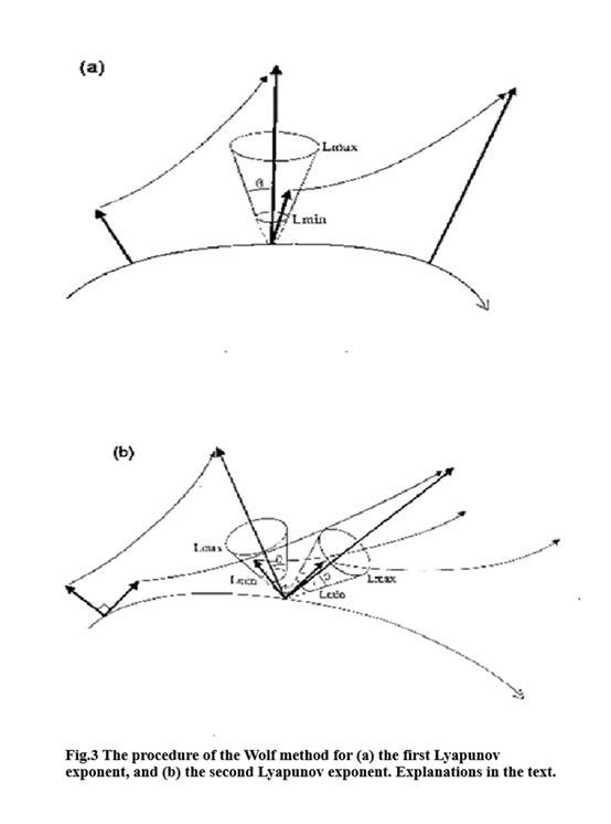
The following procedures were used for the recorded data embedded in 4-dimensional dynamical system. As seen in Fig.3(a), the largest Lyapunov exponent Ai is computed as the average growth rate of length elements. The growth rate is measured for vectors not parallel to the direction of orbits. Throughout the computation a fixed evolution time T was used. A new vector is adopted for the next evolution when its tip enters in the bounded region of the four- dimensional cone with the maximum angle \(\theta\).

The boundaries of the cone, \(L_{min}\) and \(L_{max}\) are needed for a correct estimation of the exponents. If we take too small a length, we cannot obtain the convergence of the exponents because of having too small a number of data allowed. If we take too large a length, we cannot also obtain a correct exponent for a fixed T, because the evolved vector can be a result of having been folded many times. These values cannot be predetermined, so many trials are necessary to obtain suitable ones. The maximum angle limit is also necessary to avoid too skewed vectors giving rise to an incorrect estimation.

After calculating with various values of \(L_{min},\ L_{max}\) and \(\theta\), it was concluded that, for our system, the set of values \(L_{min} =3\%\) and \(L_{max} =5\%\) of the size of the attractors, and \(\theta =18^{\circ}\) can give fast convergence.

If appropriate data are not found, the vector to be evolved is dropped, turning back by one step in the procedure to choose another. If appropriate data are not found even with this procedure, we reset a fiducial point on the treyectory. If this reset is needed many times, we must judge that such a data-set cannot give a correct calculation of the Lyapunov exponents. In all data-sets, except for the cardiac data, we calculated, a ratio of such resets was at most 1% of the total number of evolutions, giving rise to covering at least six periods in average for each fiducial trajectory which is sufficient for a correct estimation of the Lyapunov exponents* Since parts of the cardiac trajectories show a fast variation, it was difficult in the estimation to keep one fiducial trajectory for a long time. We needed a 10-20% ratio of reset, so the estimated value might not show the correct Lyapunov exponent and it should rather be considered as the average local divergence rate.

As seen in Fig.3(b), \(\lambda_1+\lambda_2\) is computed as the average growth rate of area elements. The procedure is analogous to the computation of \(\lambda_1\). Two points are chosen beside the fiducial trajectory. For the length of the corresponding two vectors, the same \(L_{min}\) and \(L_{max}\) as in Fig.3(a) were adopted. Too skewed areas are also ignored, by adopting the allowed angles \(\theta \leq 18^{\circ}\) between an evolved area and a renewed area. For each evolution, the Gram-Schmidt procedure is used for keeping orthonormality.

In order to check the correctness of the above algorithm, we calculated the first and the second Lyapunov exponents in the Lorenz system. We obtained the same values as those obtained by the conventional method of Shimada and Nagashima[Shimada & Nagashima,1979], Especially, the second exponent was zero up to the second or the third digit(0.003 土 0.0097).

If orbits are sufficiently embedded into 4-dimensional phase space, it is concluded that the third exponent \(\lambda_3\) should vanish and the fourth exponent \(\lambda_4\) should take a large negative value, i.e., \(\lambda_4 \leq (\lambda_1 + \lambda_2)\). Moreover, in general, if the embedding dimension is lower than the dimension of the attractor, the degree of orbital instability would seemingly decrease. This situation could give a lower value than the actual Lyapunov exponent. Thus, the calculated exponents give the lower bounds. These considerations show that the pulsation of the capillary vessel can be described by deterministic chaos. The positive second exponent indicates the correctness of our assumption that the attractor should be described in at least 4-dimensional dynamical system.

We also calculated the empirical Lyapunov spectrum with other methods, namely, Sano-Sawada[1985] and Eckmann-Ruelle[1986] methods, increasing the embedding dimension* The largest Lyapunov exponent gives the same value as in Table 1 within the precision. However, it was quite difficult to determine whether the second exponent is zero or positive. Both Sano-Sawada and Eckman-Ruelle methods are convenient for obtaining the whole spectrum simultaneously. It is, however, still questionable whether the tangent space is correctly spanned. Especially, the assumption that the vectors in the sphere are uniformly distributed is highly questionable in our system. An elaborated algorithm will be published elsewhere[Barna & Tsuda,1991].

5. Condition dependence of observed chaos in the cardiovascular system

For various mental or physical conditions of the subjects (resting, calculating simple arithmetic, drinking, exhaustion, unrest, sleeping, reading, looking pictures, etc. for normal subjects, and resting for different psychiatric patients), we reconstructed the attractors from recorded data, and also calculated the Lyapunov exponents. The forms of chaos, the geometry and size of trajectories as well as the Lyapunov exponents were rather sensitive to those conditions, possessing basal forms specific to the individual[Fig.4(a),(b)]. Under the same condition for a subject, the successive measurements assured invariance of the forms of chaos.

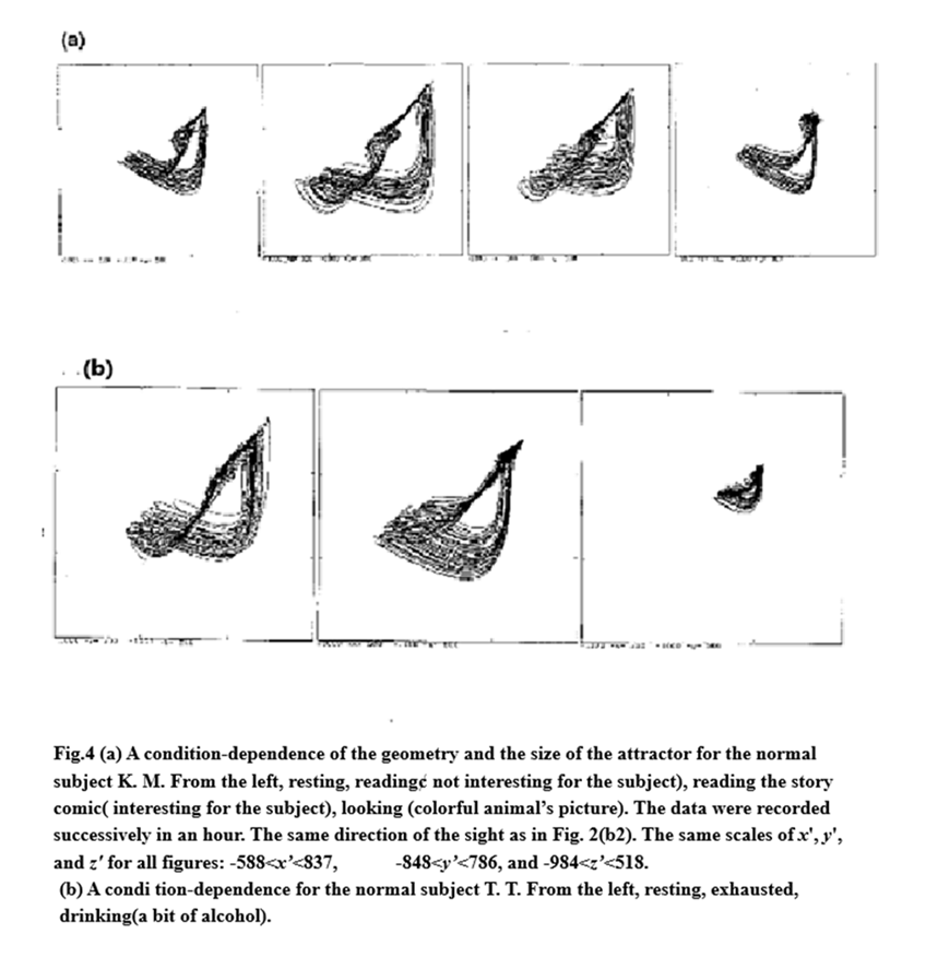
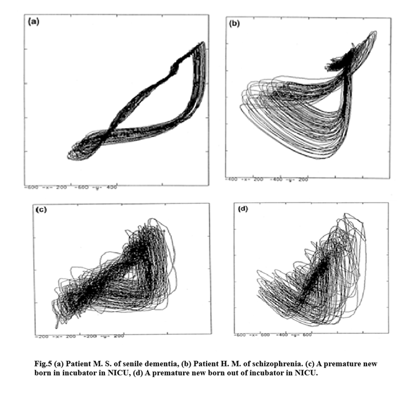
Fig.5(a)&(b) show the capillary chaos in patients of senile dementia and of schizophrenia, respectively. Features of chaos in Fig.5(a) are typical for the patients of senile dementia. However, we should stress that any features in Fig.5(b) show a specificity of schizophrenic patients. A similar attractor can appear also in normal subjects when they are out of (physical) condition.

Fig.5(c)&(d) are the data from premature newborn babies in Neonatal Intensive Care Unit (NICU): (c) a newborn in incubator, and (d) a newborn out of incubator, respectively. The data in (c) show zero as the largest Lyapunov exponent, and in (d) the largest Lyapunov exponent is near zero. Both data have not much structure. However, it should be noted that a newborn in the incubator has even less structure than a newborn out of the incubator.

Thus, the features of chaotic attractor reflect the degree of physical or mental activity(health) or the degree of maturity. This indicates that the feature change can also be an appropriate indication in the process of care of mental or physical diseases.

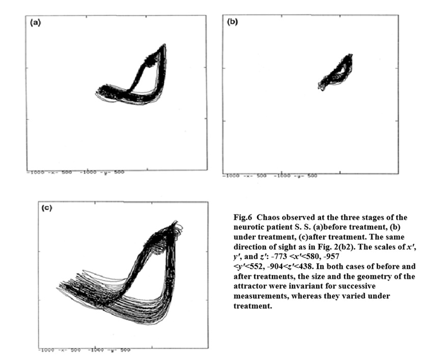
Actually, we applied our method to the rehabilitation process of a neurotic patient in order to check whether or not the chaotic representation obtained here can be utilized as an indication of the degree of recovery of mental health. Figure 6 shows reconstructed chaos at the respective stages before, under, and after treatment. A conspicuous disorder in hospitalization [Fig.6(b), see also Table 1] can be considered to stem from both a self-discord of the patient and drugs for medical treatment. After recovering mental health [Fig.6(c)] the dimension of the attractor is seemingly reduced, and there appears a complicated screw type of structure which was not so conspicuous before medical treatment [Fig.6(a)]. It should be also emphasized that the size of the attractor after the recovery becomes greater than that before treatment.

To study if the chaos observed in the capillary vessels stems from a cardiac oscillation, we made simultaneous measurements of the beating of the heart, A long-time recording of that beating in terms of the V4-induction of electrocardiograph also exhibited deterministic chaos in a subject without any heart diseases(see also [Babloyantz & Destexhe,1988; Goldberger et. 1988]), but its topology differed very much from that of the chaos of the capillary vessels (see Fig.7). Moreover, topology of the cardiac chaos is insensitive to subjects and their conditions if heart diseases such as the myocardial infarction, the atrial fibrillation, and the irregular pulse are not recognized.

6. Information Processing by the Capillary Chaos

The cardiovascular system is an information channel [Mandell, 1987] as well as the cortical nervous system. In particular, the peripheral system is considered as a control system correlating with the nervous system. Therefore, it is worth studying the information capacity of observed chaos, especially its ability for transmission of information fed from outside.

In order to study this on the experimental data, we propose a simple algorithm for computation of mutual information between the experimental data and the other dynamical system.

Let {x(n)} denote the n-th orbital point in the M-dimensional vector space. The embedding of experimental data into M-dimension allows this assignment. Let {y(n)} denote the n-th orbital point of the other data set in the M’-dimensional vector space. A set {y(n)} is supposed to have been computed in numerical simulation of the dynamical system, or obtained in another experiment. Both sets {x(n)} and {y(n)} are numbered in the order of evolution.　

We consider the following type of forced system:

where \(C\) is a matrix of coupling constants, whose elements are expressed by \(c_{ij},\ i=1, \ldots, M,\ j=1, \ldots, M’\).

Suppose that the solutions achieved in the case of \(c_{ij}=0\) for all \(i\) and \(j\) give the data sets \(\{x(n)\}\) and \(\{y(n)\} (1\leq n \leq N)\). Our aim is to construct a time series \(x'(n)\) which closely resembles a solution of Eq. (2). Choose \(x(l)\) for \(x’(1)\). In each step we compute the exact evolution from \(x’(n)\) using the term \(\mathbf{f}\left(x(t)\right)+Cy(t)\). However, since the effect of \(\mathbf{f}\) is known only for the elements of the data set \(\{x(n)\}\), we substitute the nearest element of this set for the exact evolution.

The procedures can be written as follows:

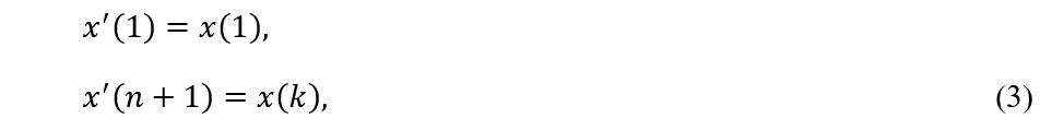
where \(x(k)\) satisfies

Divide both \(\{x’(n)\}\) and \(\{y(n)\}\) into \(m\) cells. Find the probability \(p_i (i=1, 2, \cdots, m)\) of \(\{x’(n)\}\) entering in the \(i\)-th cell, and the conditional probability \(p_{ji}^{(f)} (i =1, \cdots, m,\ j=1, …, m)\) that \(\{x'(n)\}\) enters in the \(i\)-th cell at time \(k + t\) under the condition of \(\{y(n)\}\) entering in the \(j\)-th cell at time \(k\). Then, one can define the time dependent mutual information [Matsumoto & Tsuda,1985,1987,1988] as follows:

This quantity indicates a time course of shared information between two data sets \(\{x'(n)\}\) and \(\{y(n)\}\), in other words, information transmitted from \(\{y(n)\}\) to \(\{x’(n)\}\), since the coupling is unidirectional in the present case.

In order to see the time course of information transmission in the simplest case, let us suppose that \(c_{kl}=c\delta_{kl}\), where c is a constant and the probability \(p_i\) and \({p_{ji}}^{(t)}\) are calculated in terms of only the first component of both \(\{x'(n)\}\) and \(\{y(n)\}\). To see the relevance of the algorithm Eq. (3), we calculated the mutual information , Eq. (4), in the Lorenz chaos forced by another Lorenz chaos in two ways, i.e., by means of the above algorithm and by the equations of motion. The computed system is given in the following:

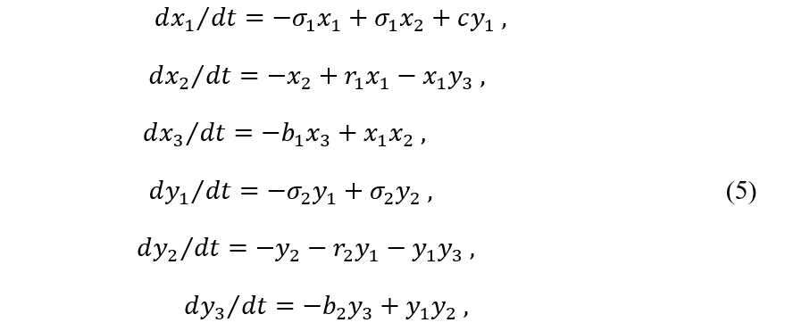
where \(\sigma_1=\sigma_2=10,\ \ r_1=r_2=28,\ \ b_1=b_2=8/3\)

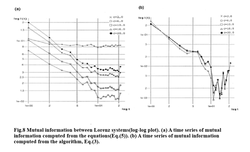
The results are shown in Fig.8, where one can see the goodness of the algorithm. The reason why \(I(t)\) is almost invariant for a change of the coupling constant is that the orbits are simply renumbered and new values can never be added by forcing. In spite of this weak point of the algorithm, as is seen in Fig.8, several cases of the coupling strength give even quantitatively good correspondence. Thus, one can adopt our algorithm as the first approximation for computing the information transmission to the experimental data from a known dynamical system or from other experimental data.

Actually, we calculated the mutual information \(I(t)\) for the capillary chaotic data which was forced by the Lorenz chaos. The capillary chaos driven by the Lorenz chaos is shown in Fig. 9(a). By this calculation, one can see the transmitted information to the capillary chaos from the Lorenz chaos. Thus, this quantity can be used to discriminate the ability of the capillary chaos of receiving information fed from outside. The results are shown in Fig. 9(b).

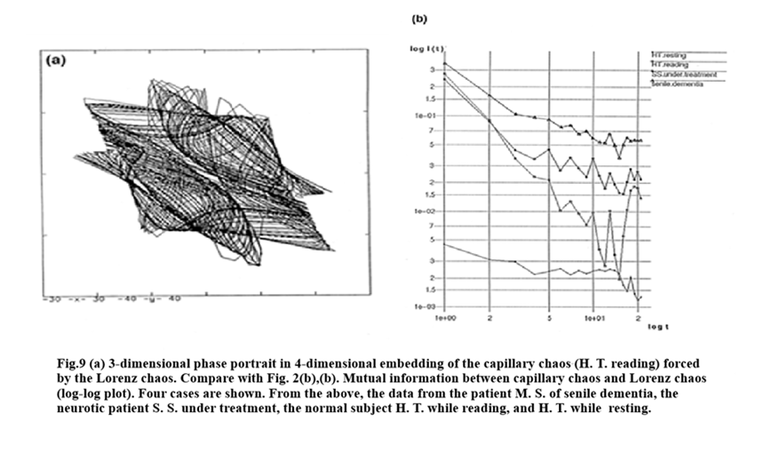
The choice of the Lorenz chaos is not essential for seeing the information processing ability of the capillary chaos. One can choose other chaotic systems or quasi¬-random noise generators as a driving system. The calculated information quantity indicates a communication ability of the capillary chaos with the Lorenz chaos. By the present algorithm, one can know, in general, the information storage capacity of any experimental data. Furthermore, adopting this algorithm to the various kinds of data sets, it will be possible to classify them in terms of their communication ability.

7. Discussions and Outlook

Two crucial hypotheses arise. The cardiovascular systems exhibited deterministic chaos in their healthy conditions. This implies that at least these systems among organs innervated by the autonomic nervous system need chaos to achieve a dynamic intelligent control [Tsuda, et αl., 1987; Tsuda, 1991(a)&(b)], here chaos buffer unexpected stimuli in terms of its inherent grammar. Relating to this notion, the definition of homeostasis might need to be corrected [Goldberger et.al., 1988].

We propose a notion of ‘homeochaotic’ state (or a state of ‘homeochaos’) in the sense that the autonomic control system can acquire intelligence and flexibility by generating deterministic chaos in its normal states. This notion was derived from the observation of chaos in the cardiovascular system reported here, but it could be easily extended to other biological systems.

A similar notion has been recently proposed by several researchers. Ikegami and Kaneko [1991] introduced the notion of ‘homeochaotic symbiotic’ network, based on the result of their symbiotic network model. Iberal [1978] proposed the notion of ‘homeokinesis’ to capture the dynamic regulations and interactions essential for the self-maintenance of biological organisms. In a similar sense, Rossler and Hudson[1990] emphasized the significance of a metabolic chaos in living systems. To denote the dynamic state achieved by chaos in the metabolic control systems, they used the notion of ‘chaotic maintenance’.

The second hypothesis is derived from the difference of the condition- sensitivity between chaos in the capillary vessels and those in the heart. Both the systems have been classified into the same category for the autonomic nerve innervation. According to our observations, however, it is plausible to think that there are at least two kinds of gates in the spinal cord. One is the gate with plasticity for innervating organs sensitive to mental or physical conditions, and the other is controlled rather automatically for innervating organs insensitive to those conditions. Only the latter should be called the autonomic nervous systems, whereas the former might be addressed as chaotically modulated autonomic nervous systems.

Acknowledgements

This work was supported by the Data Base Promoting Center, Japan. We thank Prof H. Shimizu, Dr. H. Uchimura, Mrs. K. Kiyooka and Prof K. Koketsu for helpful comments. One of the authors(I.T.) thanks Dr. G. Barna for helping to calculate the Lyapunov exponents by the Sano-Sawada and Eckman- Ruelle methods. We also thank M, Kara for critical reading of the manuscript.

References

• Babloyantz, A. & Destexhe, A.[1988], “Is the normal heart a periodic oscillator?,” Biological Cybernetics 58, 203-211.
• Babloyantz, A.[1986], “Evidence of chaotic dynamics of brain activity during the sleep cycle”, in Dimension and Entropies in Chaotic Systems, ed.. C. Mayer- Kress (Springer-Verlag, Berlin) pp.241-245.
• Barna, G. and Tsuda, I. [1991] (in preparation)
• Campbell, D. K., Crutchfield, J. P., Farmer, J. D., & Jen, E. [1984], “Experimental mathematics: The role of computation in nonlinear science,” Comm. ACM 28, 374-384.
• Eckmann, J. P., Kamphorst, S. O., Ruelle, D. & Ciliberto, S. [1986] ” Lyapunov exponents from time series,” Phy. Rev. A34, 4971-4979.
• Freeman, W. J. [1989] ” Searching for signal and noise in the chaos of brain waves,” in the Proceedings of the SanFrancisco Meeting of the American Association for the Advancement of Science(Spectrum) pp. l~10.
• Goldberger, H. L., Rigney, D. R., Mietus, J., Antman, E. M. & Greenwald, S. [1988] “Nonlinear dynamics in sudden cardiac death syndrome: Heart rate oscillations and bifurcations,” Experientia, 44, 983-987.
• Grassberger, P. & Procaccia, I. [1983a] “Characterization of strange attractors,” Phys. Rev, Lett. 50, 346-349.
• Grassberger, P. & Procaccia, I.[1983b] “Measuring the strangeness of strange attractors,” Physica D9, 189-208.
• Iberal, A. S. [1978], “A field and circuit thermodynamics for integrate physiology. I. Information to the general notions,” Am. J. Physiol, 233, 171-180.
• Ikegami, T. & Kaneko, K. 1991.
• Layne, S. P., Mayer-Kress, G., & Holzfuss, J. [1986], “Problems associated with dimensional analysis of dlectroencephalogram Data,” in Dimensions and Entropies in Chaotic Systems, ed. G. Mayer-Kress (Springer-Verlag, Berlin) pp. 246-256.
• Mandell, A. J. [1987] “Dynamical complexity and pathological order in the cardiac monitoring problem,” Physica D27, 235-242.
• Matsumoto, K. & Tsuda, I. [1985] “ Information theoretical approach to noisy dynamics,” J. Phys. A18, 3561-3566.
• Matsumoto, K. & Tsuda, I. [1987] “Extended information in one-dimensional maps,” Physica D26, 347-357.
• Matsumoto, K. and Tsuda, 1. [1988] “Calculation of information flow rate from mutual information,” J. Phys. A21, 1405-1414.
• Miyazaki, K. & Ishihara, K. [1989] Four~dimensional Graphics – Towards high dimensional CG (Asakura-shoten, in Japanese).
• Packard, N. H., Crutchfield, J. P., Farmer, J. D., & Shaw, R. S. [1980], “Geometry from a time series,” Phys. Rev. Lett. 45, 712-715.
• Rapp, P. E. et al. [1980] “ Oscillations and chaos in cellular metabolism and physiological systems,” in Chaos, ed. A. V. Holden (Manchester Univ. Press) pp 179-208.
• Rapp, P. E. et al. [1989] “Dynamics of brain electrical activity,” Brain topography, 2, 99-118.
• Rossler, 0. E. & Hudson, J. L. [1990] “Self-similarity in hyperchaotic data,” in chaos in Brain Function,, ed. E. Basar (Springer-Verlag, Berlin, Heidelberg) pp. 74-82.
• Sano, M. & Sawada, Y. [1985] “Measurement of the Lyapunov spectrum from a chaotic time series,” Phys. Rev. Lett. 55, 1082-1085.
• Schaffer, W.M., Olsen, L. F., Truty, C. L., Fulmer, S. L. & Graser, D. J. [1988] “Periodic and chaotic dynamics in childhood infection,” in From Chemical to Biological Organization, eds. Markus, M., Muller, S. C. & Nicolis, G. (Springer- Verlag) pp 331-347.
• Shimada, I. % Nagashima, T. [1979] “A numerical approach to ergodic problem of dissipative dynamical systems,” Prog. Theor. Phys. 61, 1605-1614.
• Takens, F. [1981] “Detecting strange attractors in turbulence,” Lecture Notes in Mathematics, eds. Rand, D. A. & Young, L. S., 898, 366-381 (Springer-Verlag, Berlin).
• Tsuda, L., Koerner, E. & Shimizu, H. [1987] “Memory dynamics in asynchronous neural networks,” Prog. Theor. Phys. 78, 51-71.
• Tsuda, I. [1991a] “Chaotic neural networks and thesaurus,” in Neurocomputers and Attention. eds. Holden, A. V. & Kryukov, V. L., Manchester Univ. Press, pp. 405-425.
• Tsuda, I. [1991b] “Chaotic itinerancy as a dynamical basis of Hermeneutics in brain and mind,” World Futures 32, 167-184.
• Wolf, A., Swift, J. B., Swinney, H. L. & Vastano, J. A. [1985] “Determining Lyapunov exponents from a time series,” Physica D16, 285-317.
• Yao, Y. & Freeman, W. J. [1990] “Model of biological pattern recognition with spatially chaotic dynamics,” Neural Networks, 3, 153-170.